WARNING: The following article contains nerd speak and could cause confusion, headaches, and increased understanding of sports analytics.
One point down, three seconds left, and thirty yards to the end zone. Two shuffles left and the kicker takes his position. Is he going to make it?
Fans often wrestle with these situational questions while watching sporting events. Casual viewing conversations often turn to asking such binary queries as “Who will win?” or “Will the Patriots convert this fourth down?” However, coaches and executives assembling rosters have to answer the harder questions before these game situations (e.g. is this kicker good enough to make the team?). To do this, the sports doctor would prescribe evaluation tactics a little more thorough than banter around the living room. Bayesian statistics attacks this problem in a more trustworthy way, representing a method sports teams are increasingly turning to for such problems.

Bayesian statistics helps approach player evaluation in a direct way. It provides a straightforward way to answer questions like the aforementioned “Is this kicker good enough to make the team?” Armed with simply a sample of data (potentially from a tryout) and knowledge for what performance traits make a player “good enough,” coaches can easily make such a decision. How? Assume one knows that good kickers at football camps make 74% of field goals from exactly fifty yards* and bad ones make 30% of such kicks. If it’s equally likely your previous evaluations would result in a good kicker coming to camp as a bad one, then the below outlines how a coach may go about gathering confidence in a kicker’s skill level.
If a kicker makes his first three kicks from fifty yards, using Bayesian statistics, you know that there’s a 94%** chance the kicker is good. Therefore, even though it appears the kicker is good by the eye test, with a 6% chance he’s not, you may want him to take a few more kicks. How many more? To answer this, first you can calculate the number of kicks in a row the kicker must make for there to be a 99% chance he’s good. In this case that number is 6 kicks.*** For more details on methodology or how to use Bayesian statistics, see info at the bottom of this article. However, the important takeaway is that Bayes’ theorem provides a reliable and consistent evaluation method that uses data and probability effectively.
While important to understand there are quite a few confounding variables in these assessments, drawing conclusions from Bayesian statistics provides useful input for player analysis. Other valuable inputs include psychology tests (measuring a player’s ability to handle the pressures/environment change that accompanies transitioning teams/leagues) and the eye test, but these are more prone to bias. As sports leans more and more on big data, optimization, and machine learning, it is valuable for fans of the game to understand how decisions are (and should be) made. If my kicker is stepping up for the game-winning kick, I could only remain calm knowing the legwork was put in for proper evaluation and data supports my decision to opt for this player.

*NFL kickers were 56.7% successful on in-game field goals of 50 yards or more in the 2017 regular season according to ESPN, so this seems reasonable.
**((% chance kicker is good) x (chance a good kicker makes all three))
+((% chance kicker is bad) x (chance a bad kicker makes all three)) = .5*(.74^3) + .5*(.30^3) = 0.216 –> (.74^3)*.5/.216 = 93.8%
***Start with the last part of ** above and solve for 99 –> 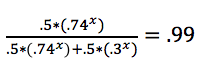
1 / .99 = 1 + (.3x)/(.74x)
0.01 = (.3/.74)x
ln (0.01) = x*ln(.3/.74)
x= 5.1 –> so won’t quite be 99% sure at just 5 kicks in a row made to start
Methods
- Predicted Event Outcomes – Situational Questions
To determine will or won’t something happen?
(kn)*pk*qn-k where (i) q = 1 – p
(ii) p = probability a single independent event occurs
Reminder: (kn)= (iii) n = number of attempts (i.e. sample size)
n!k! (n-k)! (iv) k = number of predicted successes
Example:
There’s a 95% chance our kicker makes extra points, and we are expecting a high
scoring game where we score five touchdowns tomorrow. What is the probability that he makes at least four?
(45)*.954*.051 =5*4*3*2*1(4*3*2*1)*1*.95*.95*.95*.95*.05 = 20.4% he makes 4
(55)*.955*.050 =5*4*3*2*15*4*3*2*1*.95*.95*.95*.95*.95*1 = 77.4% he makes 5
77.4+20.4 = 97.8% chance he makes at least 4 - Bayesian Statistics
What are the chances x is true given a set of observations?
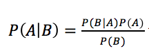 where P(B) ≠ 0
Example:
When tested for steroids, 95% of players taking them test positive and 1% of those not taking errantly test positive. If anonymous polling shows 10% of players take steroids, what is the probability a randomly selected player who tested positive took steroids?
A = took steroids
B = test positive
P(B) = .95 * .1 + .01*.9 = .104 P(B|A) = .95 P(A) = .1
Bayes: (.95*.1/.104) = 91.3%
91.3% chance that that player took steroids
Similar Topics: Bayesian Networks & Hierarchical Modeling, Markov Chain Monte Carlo, Spatial Data, Machine Learning
Awesome post! Keep up the great work! 🙂
It’s hard to find well-informed people about this topic, but
you seem like you know what you’re talking about! Thanks